Neuro-evolutionary algorithms in reinforcement learning.

October 26, 2020

Algorithms for evolutionary computation, which simulate the method of action to unravel optimization problems, are a good tool for locating high-performing reinforcement-learning approaches. Because they’ll automatically find good representations, handle continuous action spaces, and deal with partial observability. This article surveys research on the appliance of evolutionary computation to reinforcement learning, overviewing methods for evolving neural-network topologies and weights, hybrid methods that also use temporal difference methods for multi agent settings.

Reinforcement Learning:

A core topic in machine learning is that of sequential decision-making. this is often the task of deciding, from experience, the sequence of actions to perform in an uncertain environment so as to realize some goals. Sequential decision-making tasks cover a large range of possible ⊕
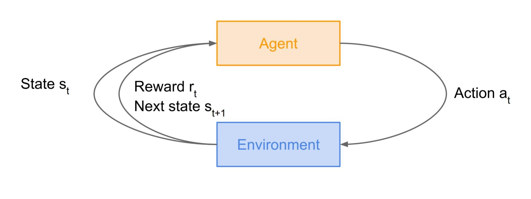
Fig 1 : RL environment (images are taken from the slides of Stanford CS231 course) applications with the potential to impact many domains, like robotics, healthcare, smart grids, finance, self-driving cars, and plenty of more. Inspired by behavioural psychology (see e.g., Sutton, 1984), reinforcement learning (RL) proposes a proper framework to the present problem. the most idea is that a synthetic agent may learn by interacting with its environment, similarly to a biohazard. Using the experience gathered, the factitious agent should be able to optimize some objectives given within the variety of cumulative rewards. This approach applies in essence to any sort of ⊕
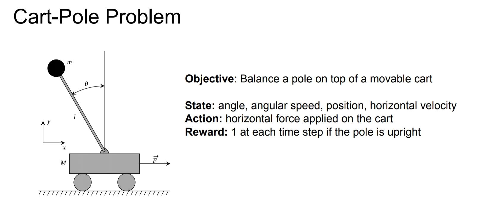
Fig 2: Cart-Pole Problem (from cs231n) sequential decision-making problem looking forward to past experience. The environment is also stochastic, the agent may only observe partial information about this state, the observations is also high dimensional (e.g., frames and time series), the agent may freely gather experience within the environment or, on the contrary, the info is also is also constrained (e.g., not access to an accurate simulator or limited data).

One ⊕
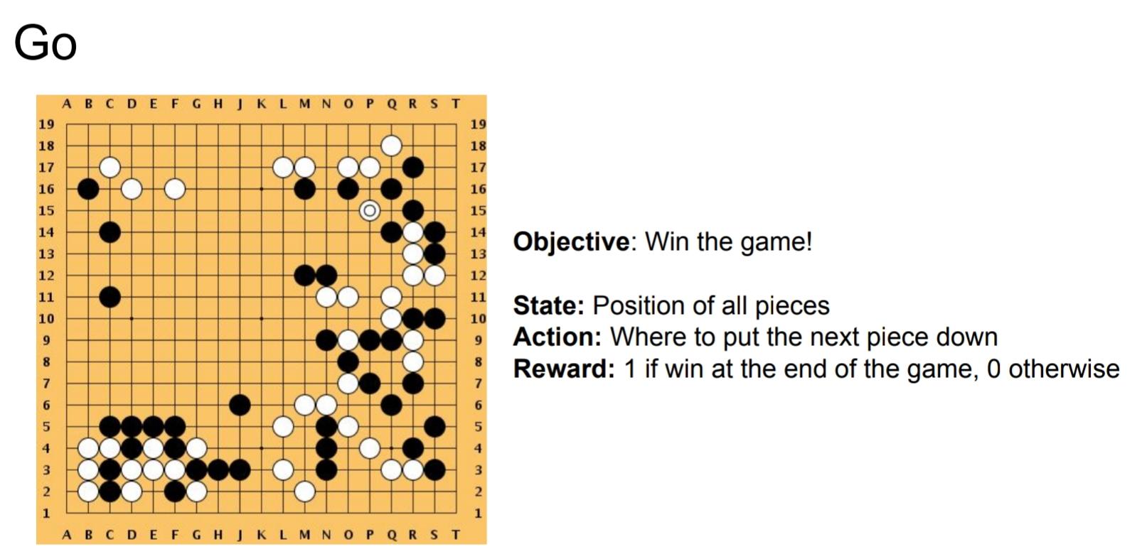
Fig 3 : GO game (from cs231n) of the challenges that arise in reinforcement learning, and not in other forms of learning, is that the trade-off between exploration and exploitation. To get lots of reward, a reinforcement learning agent must prefer actions that it’s tried within the past and located to be effective in producing reward. But to get such actions, it’s to undertake actions that it’s not selected before. The agent must exploit what it’s already experienced so as to get reward, but it also must explore so as to form better action selections within the future.

The Optimization problem:

Machine learning models are in essence function approximators. Whether it’s classification, regression or reinforcement learning, the top goal is nearly always to search out a function that maps computer file to output data. you employ the training data to infer the parameters and hyperparameters and verify with the test data whether the approximated function performs well on unseen data. The inputs are often manually defined features or information (images, text, etc.) and also the outputs are either classes or labels in classification, real values in regression and actions in reinforcement learning. For this blog post we are going to limit the kind of function approximators to deep learning networks, yet the identical discussion applies to other models. The parameters that require to be inferred thus correspond to the weights and biases within the network. ‘Performing well on train and test data’ is expressed through objective measures, like the log loss for classification, the mean squared error (MSE) for regression and also the reward for reinforcement learning. The core problem is thus finding the parameter settings that leads to very cheap loss or the very best reward. Simple! Given an optimization objective, i.e. the loss or the reward, that has to be optimized as a function of the networks parameters the goal is thus to tweak the parameters in such how that the optimization objective is minimized or maximized.

Gradient Descent:

This optimization algorithm is recruited to seek out values that reduce the value function. this is often done through the calculation of a gradient value, that’s utilized to pick out values at each step that finds the local minimum of a price function. The negative of the gradient is employed to seek out the local minimum. Essential to gradient descent is that the computation of proper gradients that propel you towards a decent solution. In supervised learning, it’s possible to get ‘high quality gradients’ with relative ease through the labelled datasets. In reinforcement learning however, you’re only given a sparse reward, because the random initial behaviour won’t cause a high reward. additionally this reward only occurs after a pair of actions. While the loss in classification and regression could be a relatively good proxy for the function you’re trying to approximate, the reward in reinforcement learning is usually not a awfully good proxy of the behaviour or function you wish to be told.

Evolution Strategies (ES):

Algorithms for evolutionary computation, sometimes known as genetic algorithms (Holland, 1975; Goldberg, 1989), are optimization methods that simulate the process of natural selection to find highly fit solutions to a given problem. Typically the problem assumes as input a fitness function f : C → R that maps C, the set of all candidate solutions, to a real-valued measure of fitness. The goal of an optimization method is to find c∗ = argmaxc f(c), the fittest solution⊕
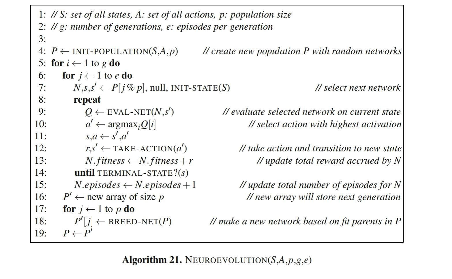
Image taken from ‘Reinforcement learning State of the Art’ book . In some cases, the fitness function may be stochastic, in which case f(c) can be thought of as a random variable and c∗ = argmaxc E[ f(c)].

Neuroevolution, genetic algorithms, evolution strategies all revolve round the concept of genetic evolution. after you do genetic optimization within the context of DNN optimization, you begin from an initial population of models. Typically, a model is randomly initialized, and a number of other offspring are derived supported this primary model. within the case of DNN’s, you initialize a model (as you normally do), and you add small random vectors, sampled from an easy distribution, to the parameters. This ends up in a cloud of models, which all reside somewhere on the optimization surface. Note that this can be the primary important distinction with gradient descent. you begin (and still work) with a population of models, rather than one (point) model.

Starting from this original population,⊕
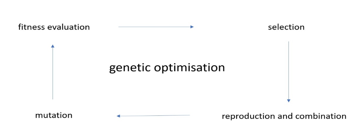
Fig 2 Overview of Genetic optimization the genetic optimization cycles start. In what follows i’ll describe genetic optimization within the context of evolution strategies (ES). Evolution strategies, genetic algorithms, etc. all have slightly different approaches on how genetic optimization is performed.

Trade-offs between ES and RL:

ES enjoys multiple advantages over RL algorithms (some of them are a touch technical):

No need for backpropagation: ES only requires the passing game of the policy and doesn’t require backpropagation (or value function estimation), which makes the code shorter and between 2-3 times faster in practice. On memory-constrained systems, it’s also not necessary to stay a record of the episodes for a later update. there’s also no must worry about exploding gradients in RNNs. Lastly, we are able to explore a way larger function class of policies, including networks that don’t seem to be differentiable (such as in binary networks), or ones that include complex modules (e.g. pathfinding, or various optimization layers).

Highly parallelizable: ES only requires workers to speak some scalars between one another, while in RL it’s necessary to synchronize entire parameter vectors (which are often several numbers). Intuitively, this can be because we control the random seeds on each worker, so each worker can locally reconstruct the perturbations of the opposite workers. Thus, all that we’d like to speak between workers is that the reward of every perturbation. As a result, we observed linear speedups in our experiments as we added on the order of thousands of CPU cores to the optimization.

Higher robustness: Several hyperparameters that are difficult to line in RL implementations are side-stepped in ES. for instance, RL isn’t “scale-free”, so one can do very different learning outcomes (including a whole failure) with different settings of the frame-skip hyperparameter in Atari. As we show in our work, ES works about equally well with any frame-skip.

Structured exploration: Some RL algorithms (especially policy gradients) initialize with random policies, which frequently manifests as random jitter on spot for a protracted time. This effect is mitigated in Q-Learning thanks to epsilon-greedy policies, where the max operation can cause the agents to perform some consistent action for a long time (e.g. holding down a left arrow). this can be more likely to try and do something in an exceedingly game than if the agent jitters on spot, as is that the case with policy gradients.

Credit assignment over while scales: By studying both ES and RL gradient estimators mathematically we are able to see that ES is a horny choice especially when the amount of your time steps in an episode is long, where actions have long-lasting effects, or if no good value function estimates are available. Conversely, we also found some challenges to applying ES in practice. One core problem is that so as for ES to figure, adding noise in parameters must cause different outcomes to get some gradient signal. As we elaborate on in our paper, we found that the utilization of virtual batchnorm can help alleviate this problem, but further work on effectively parameterizing neural networks to own variable behaviours as a function of noise is important.

Conclusion:

Will neuroevolution be the longer term of deep learning? Probably not, but I do believe it shows great promises for hard optimisation problems, like in reinforcement learning scenario’s. additionally, I feel a mixture of neuroevolution and gradient descent methods will result in a major improvement in RL performance. One downside of neuroevolution is that the massive amounts of compute power that are required so as to coach these systems. The re-emergence of neuroevolution is one more example that old algorithms combined with modern amounts of computing can work surprisingly well.

References:

Richard S. Sutton and Andrew Barton. Reinforcement learning: An Introduction.

Macro Wiering. Reinforcement Learning: State-of-the-Art.

Felipe Petroski Such, Vashisht Madhavan, Edoardo Conti, Joel Lehman, Kenneth O. Stanley, Jeff Clune. Deep Neuroevolution: Genetic Algorithms Are a Competitive Alternative for Training Deep Neural Networks for Reinforcement Learning.

Joel Lehman, Jay Chen, Jeff Clune, Kenneth O. Stanley. Safe Mutations for Deep and Recurrent Neural Networks through Output Gradients.

Xingwen Zhang, Jeff Clune, Kenneth O. Stanley. On the Relationship Between the OpenAI Evolution Strategy and Stochastic Gradient Descent.

Joel Lehman, Jay Chen, Jeff Clune, Kenneth O. Stanley. ES Is More Than Just a Traditional Finite-Difference Approximator.

Edoardo Conti, Vashisht Madhavan, Felipe Petroski Such, Joel Lehman, Kenneth O. Stanley, Jeff Clune. Improving Exploration in Evolution Strategies for Deep Reinforcement Learning via a Population of Novelty-Seeking Agents.

Tim Salimans, Jonathan Ho, Xi Chen, Szymon Sidor, Ilya Sutskever. Evolution Strategies as a Scalable Alternative to Reinforcement Learning.